5.26. THE BUTTERFLY EFFECT
A simulation model with Vensim
 When a simulation model is created, the system's elements often behave in a surprising and even totally unexpected way. The changes we make to the initial conditions can also result in opposite or very different effects from those anticipated. Moreover, small changes in initial values may result in considerable differences in the behaviour of the system's elements.
Perhaps unknowingly we create a simulation model with a structure and a relationship among variables such that, under specific conditions, it behaves in a way known as chaos. A definition of chaos says that it is "an aperiodic behaviour in a deterministic system that is very sensitive to initial conditions".
The simulation model does not have to be very complex with a lot of variables, parameters and feedback. Numerous studies have shown that with three differential equations and with one of them being non-linear, we have the conditions needed for the system to have chaotic behaviour under certain conditions.
In the last few decades of the twentieth century, Chaos Theory attracted considerable interest since it showed the interconnected reality that surrounds and fills us with feedback loops, where each constituent element acts to modify the behaviour of the environment that surrounds it, but does not do so independently. Instead, it obeys an integrated behaviour of the whole. This theory is particularly useful to tackle the study of social phenomena, which are always complex and difficult to solve in terms of linear cause-effect relationships.
Fortunately, there are examples of physical phenomena or purely mathematical systems, such as the forced pendulum- a physical phenomenon or a third order differential equation- a mathematical model that makes it easier to understand chaotic behaviour before modelling much more difficult situations, such as social phenomena. We have an even more famous example, because of its cinematographic repercussions, from the work of meteorologist Edward Lorenz who over forty years ago constructed a three differential equation system to model meteorological behaviour in a simple way. He obtained a surprising as well as eye-catching response commonly known as the "Butterfly Effect".
In the 1960s, meteorologist Edward Lorenz began a series of investigations focused on solving the problem of meteorological prediction. Working in a two-dimensional rectangular atmosphere whose lower zone is at a higher temperature than the upper zone and using continuity equations, amount of movement and thermal balance, he developed a simplified system formed by three differential equations.
It is important to observe that there are three differential equations that have two nonlinearities, the products " x.y " and " x.z ". That is why this system meets the conditions for chaotic behaviour to appear in its state variables ("state variables" are called Levels in System Dynamics).
We can represent these equations with a dynamic simulation model. Nevertheless, it is important to keep in mind that the previous equations are the result of a regular process when analysing physical and chemical phenomena. It consists of adimensionalising variables. The result of this process is the appearance of groups of parameters (for example, characteristic density, viscosity, longitude) known as adimensional numbers, which establish relationships between the driving forces of change in the system being studied; in other words, its dynamics.
The created model is made up of three Levels called Convective Flow, Horizontal Temperature Difference and Vertical Temperature Difference, which depend on their respective Flows, which are: Convective Flow Variation, Horizontal Temperature Variation and Vertical Temperature Variation. In addition, there are three adimensional parameters: the Prandtl Number, which establishes a relationship between the viscosity and thermal conductivity of the fluid, the Rayleigh Number, which quantifies heat transmission in a fluid layer through internal heat radiation and Height, which represents the thickness of the layer being studied.
The model basically establishes the relationship between the convective flow and the variations in temperature of the air mass, which is complex in itself since a difference in temperature produces a convective flow and this flow, in turn, modifies the difference in temperature, all this contingent on the properties of the medium studied, such as viscosity, density or thermal conductivity, which are grouped together in adimensional numbers which appear as model parameters.
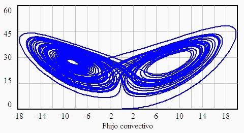
In this exercise, strictly speaking, what we are doing is making a graph of phase space. Phase space is the mathematical space created by the variables that describe a dynamic system. Each point of the phase space represents a possible state of the system. The system's evolution in time is represented with a trajectory in the phase space.
Phase space study is of special interest. The dissipative systems have regions of phase space toward which the trajectories which originate from a specific region called the "attractor basin" converge. There are predictable attractors with a simple structure, such as the point or the limit cycle. But there are other attractors known as strange attractors in which small differences in the initial positions lead to positions which completely diverge. This is precisely the case of the Lorenz attractor with its peculiar form similar to that of a butterfly.
When a simulation model is created, the system's elements often behave in a surprising and even totally unexpected way. The changes we make to the initial conditions can also result in opposite or very different effects from those anticipated. Moreover, small changes in initial values may result in considerable differences in the behaviour of the system's elements.
Perhaps unknowingly we create a simulation model with a structure and a relationship among variables such that, under specific conditions, it behaves in a way known as chaos. A definition of chaos says that it is "an aperiodic behaviour in a deterministic system that is very sensitive to initial conditions".
The simulation model does not have to be very complex with a lot of variables, parameters and feedback. Numerous studies have shown that with three differential equations and with one of them being non-linear, we have the conditions needed for the system to have chaotic behaviour under certain conditions.
In the last few decades of the twentieth century, Chaos Theory attracted considerable interest since it showed the interconnected reality that surrounds and fills us with feedback loops, where each constituent element acts to modify the behaviour of the environment that surrounds it, but does not do so independently. Instead, it obeys an integrated behaviour of the whole. This theory is particularly useful to tackle the study of social phenomena, which are always complex and difficult to solve in terms of linear cause-effect relationships.
Fortunately, there are examples of physical phenomena or purely mathematical systems, such as the forced pendulum- a physical phenomenon or a third order differential equation- a mathematical model that makes it easier to understand chaotic behaviour before modelling much more difficult situations, such as social phenomena. We have an even more famous example, because of its cinematographic repercussions, from the work of meteorologist Edward Lorenz who over forty years ago constructed a three differential equation system to model meteorological behaviour in a simple way. He obtained a surprising as well as eye-catching response commonly known as the "Butterfly Effect".
In the 1960s, meteorologist Edward Lorenz began a series of investigations focused on solving the problem of meteorological prediction. Working in a two-dimensional rectangular atmosphere whose lower zone is at a higher temperature than the upper zone and using continuity equations, amount of movement and thermal balance, he developed a simplified system formed by three differential equations.
It is important to observe that there are three differential equations that have two nonlinearities, the products " x.y " and " x.z ". That is why this system meets the conditions for chaotic behaviour to appear in its state variables ("state variables" are called Levels in System Dynamics).
We can represent these equations with a dynamic simulation model. Nevertheless, it is important to keep in mind that the previous equations are the result of a regular process when analysing physical and chemical phenomena. It consists of adimensionalising variables. The result of this process is the appearance of groups of parameters (for example, characteristic density, viscosity, longitude) known as adimensional numbers, which establish relationships between the driving forces of change in the system being studied; in other words, its dynamics.
The created model is made up of three Levels called Convective Flow, Horizontal Temperature Difference and Vertical Temperature Difference, which depend on their respective Flows, which are: Convective Flow Variation, Horizontal Temperature Variation and Vertical Temperature Variation. In addition, there are three adimensional parameters: the Prandtl Number, which establishes a relationship between the viscosity and thermal conductivity of the fluid, the Rayleigh Number, which quantifies heat transmission in a fluid layer through internal heat radiation and Height, which represents the thickness of the layer being studied.
The model basically establishes the relationship between the convective flow and the variations in temperature of the air mass, which is complex in itself since a difference in temperature produces a convective flow and this flow, in turn, modifies the difference in temperature, all this contingent on the properties of the medium studied, such as viscosity, density or thermal conductivity, which are grouped together in adimensional numbers which appear as model parameters.
In this exercise, strictly speaking, what we are doing is making a graph of phase space. Phase space is the mathematical space created by the variables that describe a dynamic system. Each point of the phase space represents a possible state of the system. The system's evolution in time is represented with a trajectory in the phase space.
Phase space study is of special interest. The dissipative systems have regions of phase space toward which the trajectories which originate from a specific region called the "attractor basin" converge. There are predictable attractors with a simple structure, such as the point or the limit cycle. But there are other attractors known as strange attractors in which small differences in the initial positions lead to positions which completely diverge. This is precisely the case of the Lorenz attractor with its peculiar form similar to that of a butterfly.
|

 See the book